Quantified Self-Tracking Shoe Insole

From September 2018 until April 2019, I completed my senior thesis project as part of my Bachelor's of Science in Electrical Engineering from Harvard University. The full thesis has been archived and is available for check-out from the Harvard University library system. Below, I've extracted the most relevant excerpts with regard to project design and fabrication.

Quantified self-tracking (QST) is a recent trend in individual healthfulness in which wearable devices, including Apple Watches and Fitbits, collect data on wearers' motion and exercise patterns in everyday life for later review of personal exercise habits. Wrist-based devices are the commonly available type on the market, but some potential customers are driven away by the devices' bulkiness and aesthetic limitations.

This project involves design of a standalone, noninvasive shoe insole that collects data comparable to what a wrist-based quantified self-tracking device would be able to provide. This QST insole includes custom electrical design, mechanical design, and software.

Electrical Design

The design of the QST insole can be divided into its electrical circuitry and mechanical design. The first section on Proto 1 will cover the qualification and testing of sensors used in the final assembly. The second section focuses in on the design decisions made for the system integration Proto 2 build. The Proto 2 build brings together the electrical sensors with a processing center in a smaller package area to create a better "product" than the Proto 1 build which only has an electrical component.

Proto 1 Electrical Build

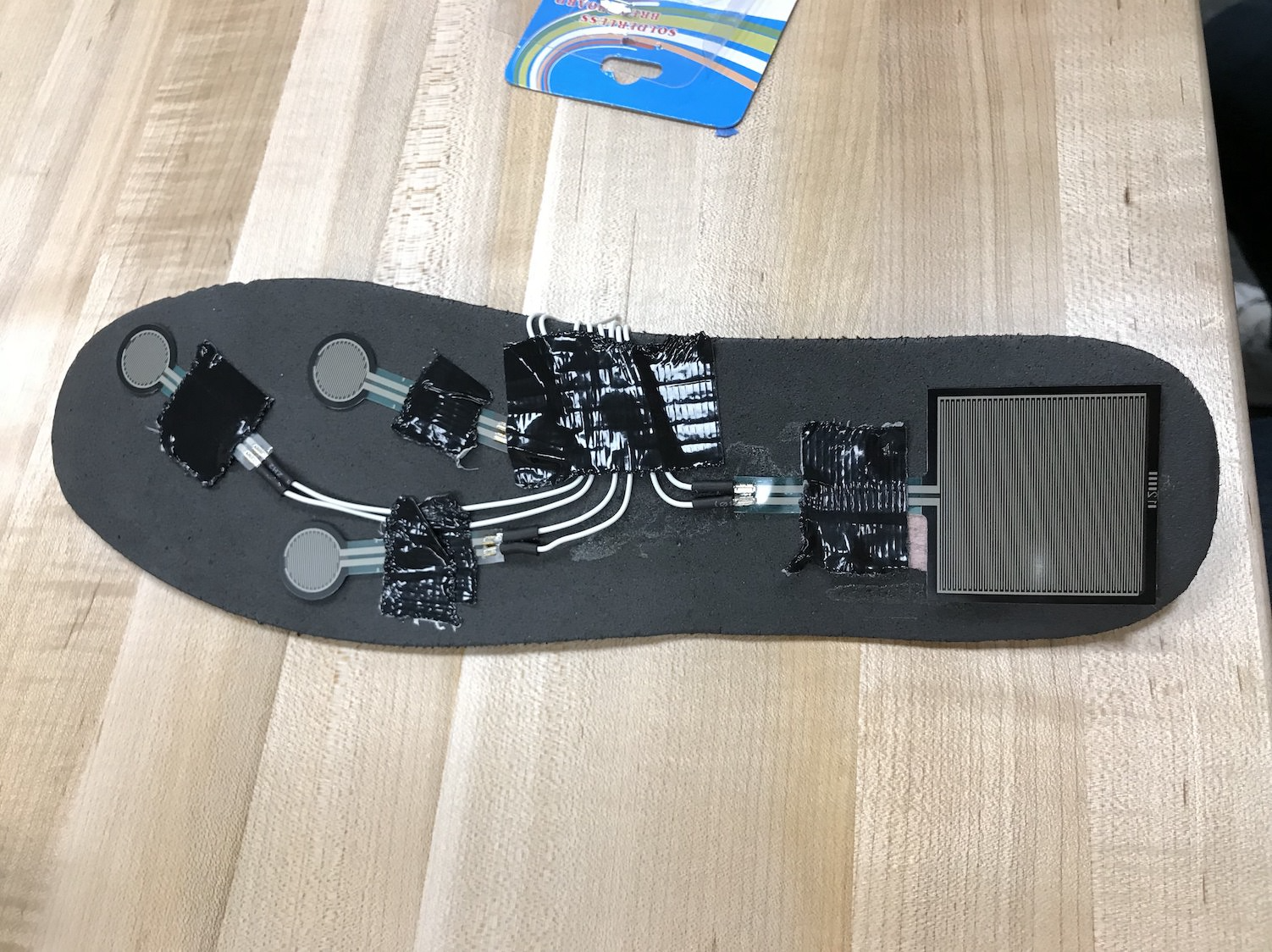
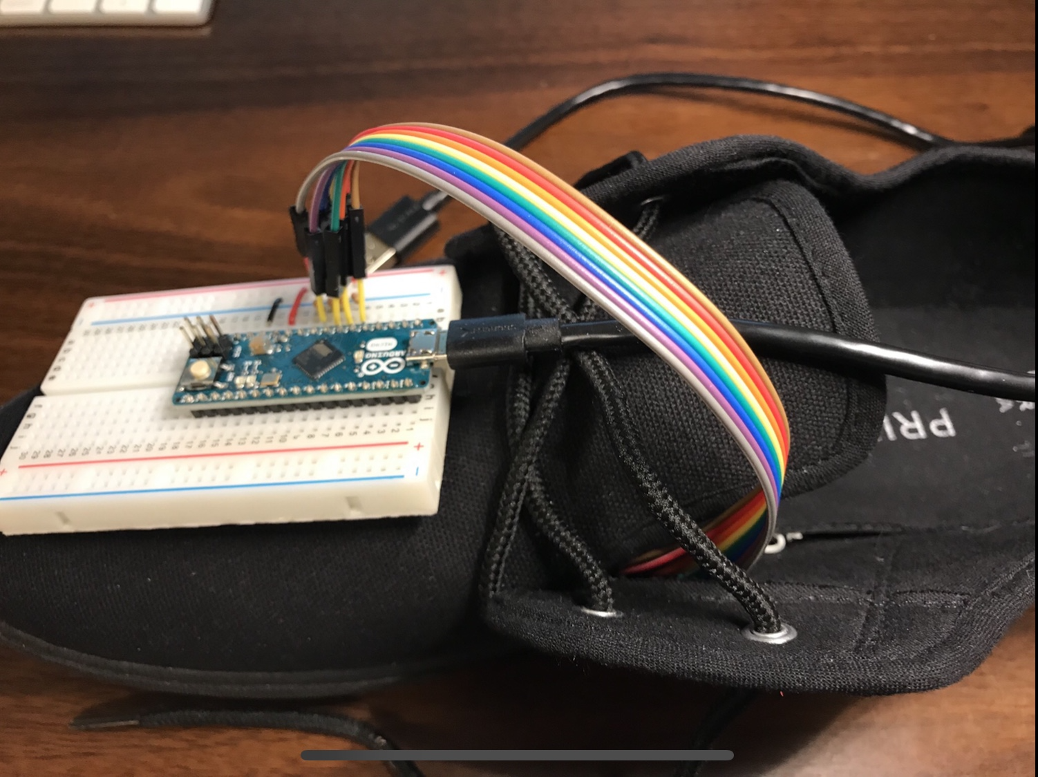
Proto 1 is a functional prototype which showcases the electrical components of the QST insole. This prototype uses wires that are manually cut to size and an Arduino to handle data processing. The onboard battery, power circuit, and processor are omitted in favor of a bulkier "processing block" meant to be carried separate from the insole, strapped to the top of the shoe containing the insole.

Sensors were tested by adhering them to the inside of the insole of a commercially-available Men's Size 10.5 fabric shoe purchased from Primark. The shoe was chosen because it was a relatively hard base underneath the insole and could be used as an inexpensive test shoe on which to do sensor validation. The goal of Proto 1 was to install sensors in conditions similar to what would be experienced in the final product and validate those sensors' performance.

A "processing block" was secured using a Velcro strap to the top of the shoe during testing. The pressure sensors could be plugged into the breadboard and the resistors on the surface could be swapped out easily while calibrating the pressure sensors. The system was robust enough to withstand regular indoor movement but could only be used outdoor under dry, controlled conditions.

A pressure sensor was required to provide data for "steps walked" as defined in the design specification. There are many sensors that are capable of measuring force or pressure, so a thorough analysis was conducted to determine the most suitable one for this application. The chosen sensor would need to provide a binary value supporting users weighing between 0lbs and 300lbs. Measurements would need to be consistent across time, with minimal variance from measurement to measurement.

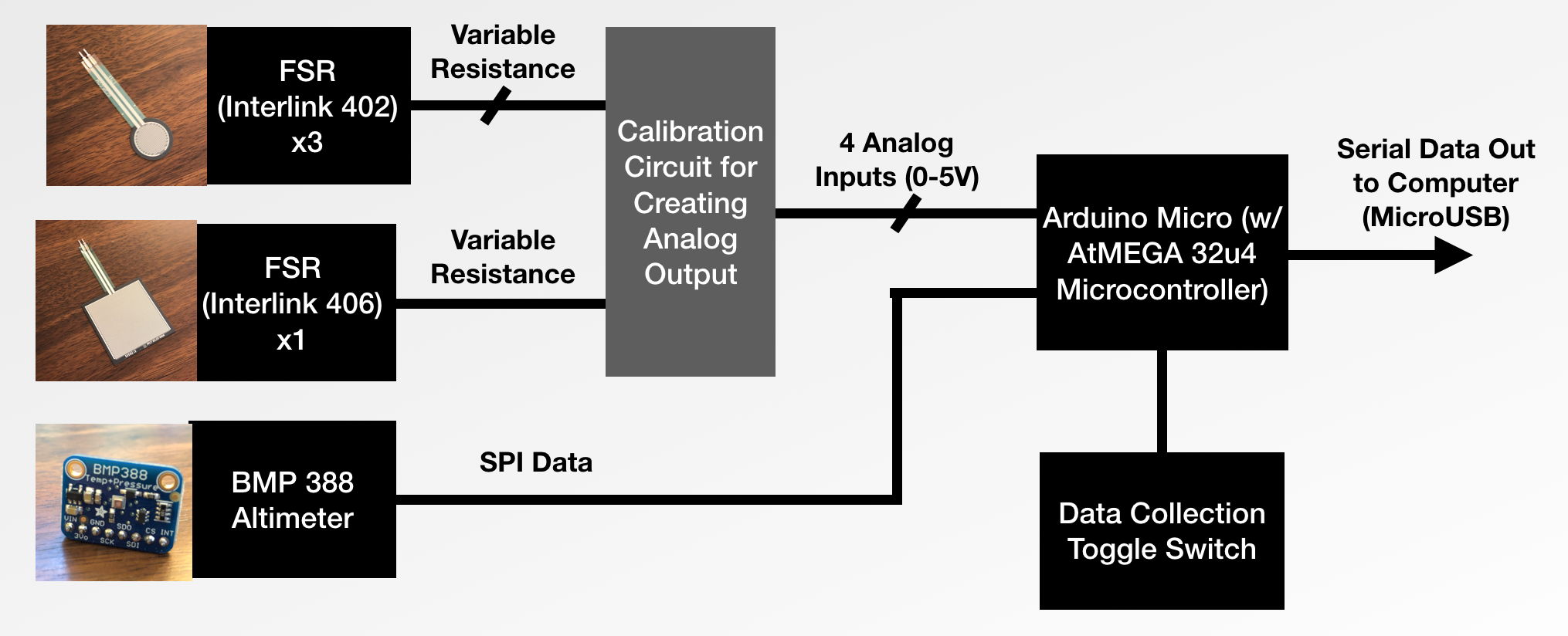
The BMP 388 Altimeter was chosen over the LIS3DH Accelerometer because it provided a much simpler data output. The purpose of the sensor was purely to measure changes in the Z altitude of the sensor, so the X and Y measurements of the accelerometer would need to be discarded. The BMP 388 streamed SPI data out and, through the implementation of a library provided with the board, that data could be converted to an integer value representing the absolute altitude relative to sea level.

For simplicity, an Arduino Micro was chosen as the central microcontroller board for the Proto 1 design. The Arduino Micro is one of the smaller Arduinos and its small form factor made it easy to plug into a breadboard for prototyping purposes. The ATmega32U4 microcontroller on the Arduino has built-in USB support which allowed for easy data-streaming.

Once data is streamed to a computer via Micro USB, it can be logged in a terminal program once a connection is opened with the correct baud rate. The program CoolTerm has the benefit of being able to write serial data to a text file for later analysis. The data for all Proto 1 tests was collected using this mechanism and stored in raw text files for later analysis.

Proto 2 Electrical Design

Five subsystems are contained within the motherboard of the Proto 2. Those five subsystems are (1) Main Microcontroller and AVR Programming Header, (2) FTDI Data Output, (3) Pressure Sensor Inputs, (4) MicroSD Card, and (5) Barometer Input.

The microcontroller chosen for the Proto 2 board was an ATtiny 44 primarily due to its small form factor and ability to satisfy the I/O pin requirements to support all necessary peripherals. The RESET pin of the microcontroller was tied to VCC via a 10k resistor. The necessary programming pins (MOSI, MISO, SCK, RST) in addition to VCC and GND were routed to a 2x3 header that allowed programming of the ATtiny 44 while it was soldered onto the board surface.

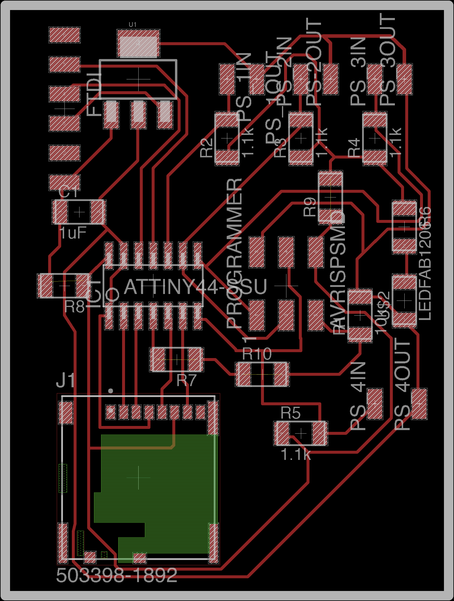
An FTDI data output was chosen as the primary means to stream data off of the board because it provided the slimmest output port in terms of Z height at only 0.1" with the 90 degree headers. The six pins for FTDI (RX, TX, RTS, CTS) and VCC and GND were routed to a 6x1 0.1" 90 degree header on the edge of the board. This positioning allowed for an FTDI cable to be connected at the boundary of the insole to stream data out up the user's leg toward a computer.

Four pressure sensor plugin points were added to the board; three faced the front for receiving the input from the inside ball, outside ball, and toe sensors, while one at the back received the input from the heel sensor. These pressure sensor plugins were female 2x1 0.1" 90 degree headers that allowed for the standard 22 gauge wire from the sensors to plug into the board directly.

The MicroSD female plugin was placed near the back of the board where it was relatively protected from the other plugins while still allowing room to access an SD card. The SD card was set up for communication over SPI protocol with MOSI and MISO pins driven from the ATtiny 44.

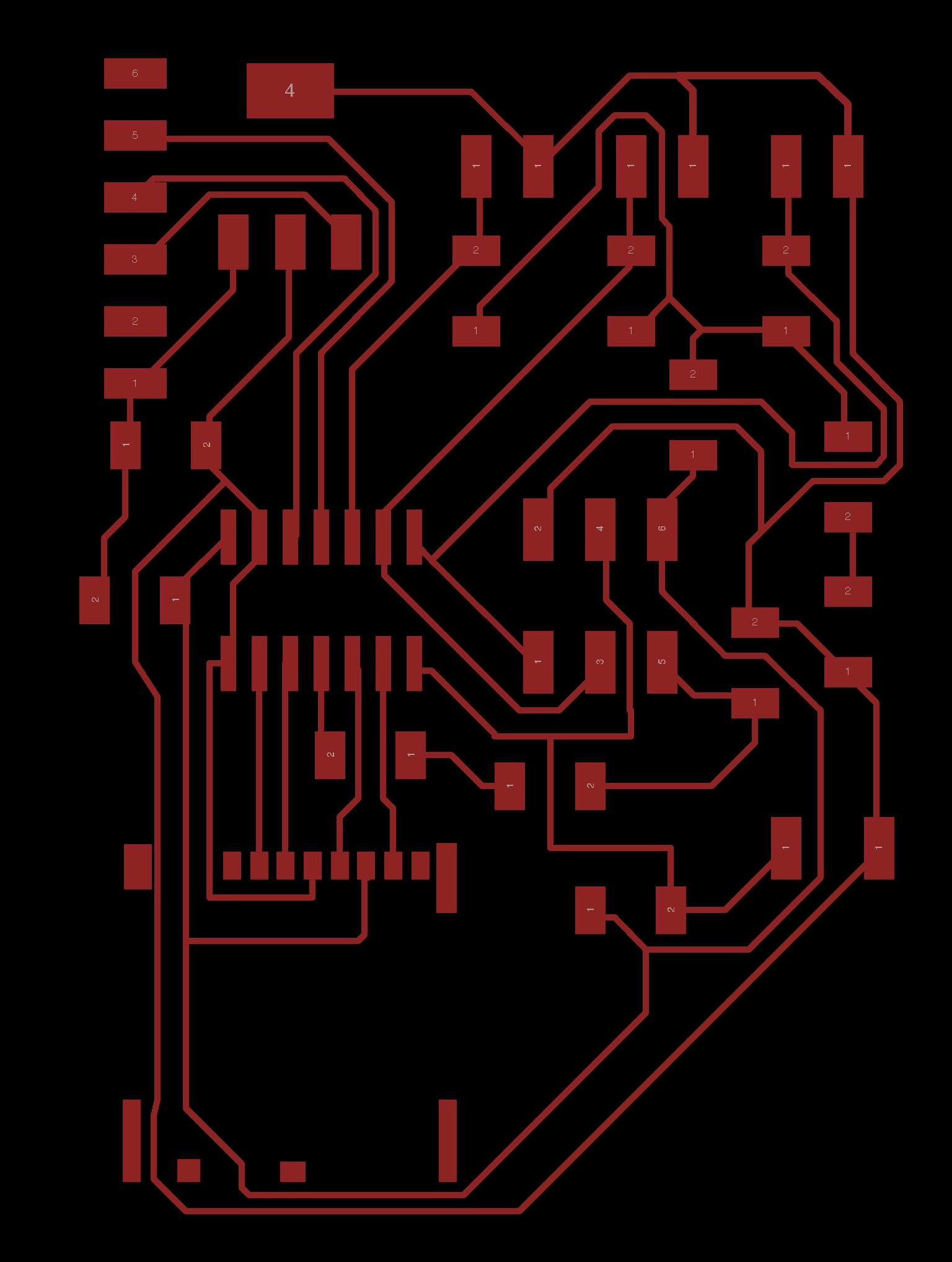
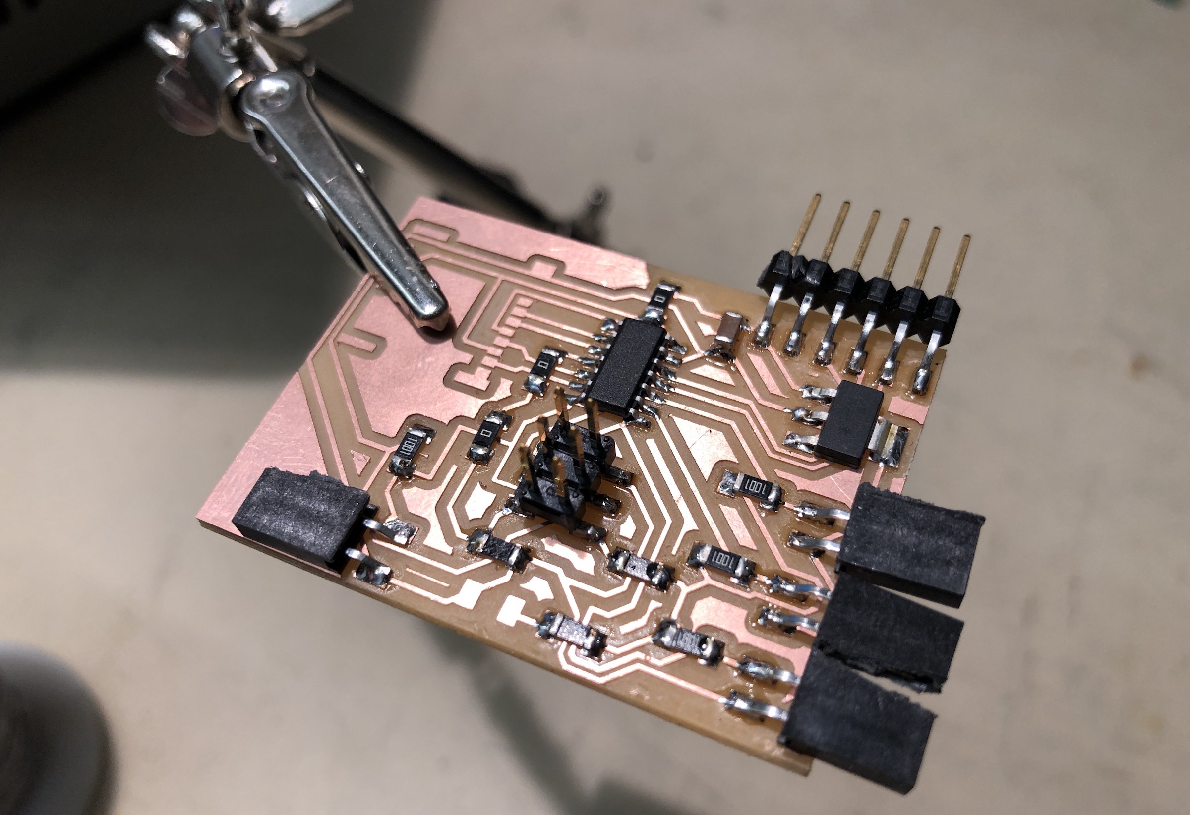
The milling machine chosen to fabricate the PCB was the monoFab SRM-20 Compact Milling Machine. The smallest end mill available was the 1/64" (15.625 mil) end mill meaning the clearance between traces would have to be at least 16 mil for every trace on the board. Trace width could not be smaller than approximately 10 mil because under this trace width, the copper on the board would be pulled up by the end mill. The board would have to be single-layer and no larger than 6" x 8" which was the available cutting area. No vias or through-hole components could be used easily as the copper only coated the surface meaning all parts had to be surface-mount.

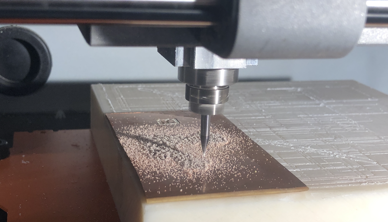
Manufacturing the board on the SRM-20 milling machine began with exporting a monochrome traces file so that a toolpath could be generated. The traces were milled using a 1/64" end mill which was just small enough to handle all of the clearances on the board. The outer dimension of the board - cutting it out of the stock material - was done with a 1/32" end mill and a separate cut file.

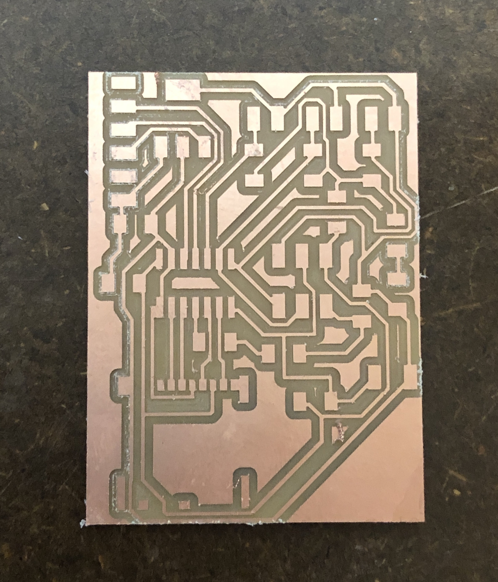
Once the board was complete, it was removed from the milling machine bed and finished with fine-grained sandpaper to remove any copper edges remaining. Visual inspection revealed no manufacturing defects and no unintended shorts between neighboring traces. The depth of the cuts into the board were consistent across the surface which indicates effective Z-axis zeroing.

The board was hand-soldered - all components were surface-mount with visible pins to make soldering possible without solder paste and more complex reflow equipment. Since milling the boards from copper meant they did not have soldermask or silkscreen, the boards were handled extremely delicately to prevent traces from being ripped off.

Mechanical Design

The customized dimensions of the main PCB and other electronics embedded in the insoles meant that a custom-designed physical insole was needed for Protos 2 and 3. The insoles were designed to be simple and based off of the dimensions of the insole used in Proto 1 with multiple layers to accommodate the different electronics.

All physical designs were produced using solid and surface modeling techniques in Autodesk Fusion 360. The physical production of the insoles was done by 3D printing the pieces using the Formlabs Form 2, a stereolithography 3D printer. The two resins used were Tough V5 and Flexible V2 resin, also from Formlabs.

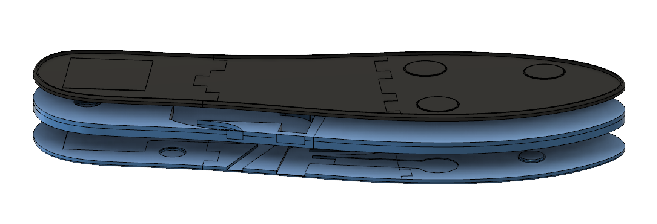
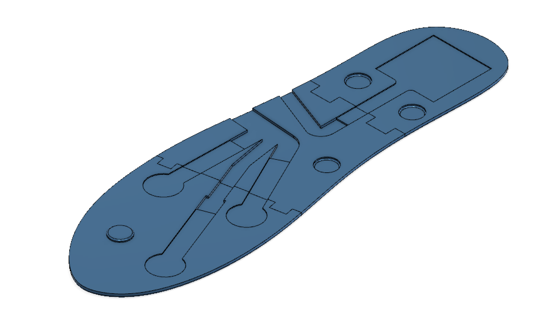
The Proto 2 physical design was intended to be the simplest possible insole shape that would support all of the relevant electronics. To maintain simplicity, no surface modeling techniques were used and the entire insole was constructed from dimensioned geometries and splines. The insole was broken into three primary layers shown below.

The base layer of the insole is 0.10" thick. This layer is where the force sensors are placed in order to ensure they have a solid base under them for accurate measurements. Three circular force sensitive resistors are placed in the front portion of the foot in a 0.02" recess corresponding to the height of the pressure sensor. There is a deeper 0.05" recess beyond the end of the pressure sensor to allow for routing of the wires from the pressure sensor back to the motherboard layer. An identical recess layout is used for the heel force sensitive resistor.

The base layer is split into three pieces to allow for manufacture on the Form 2 printer which has a build platform of only 5.7" by 5.7" by 6.9". The insole's front-to-back length is just over 10" meaning it could not be printed all as one piece. The three pieces have cut-outs to allow for alignment and puzzle-piece style fitting during assembly. Alignment nubs are also included on the top of the base layer for vertical alignment between this and the motherboard layer. The nubs are 0.5" diameter circles at a height/depth of 0.05" to allow for smooth alignment. They are placed away from the pressure sensors and not intended to concentrate the force on a particular area.

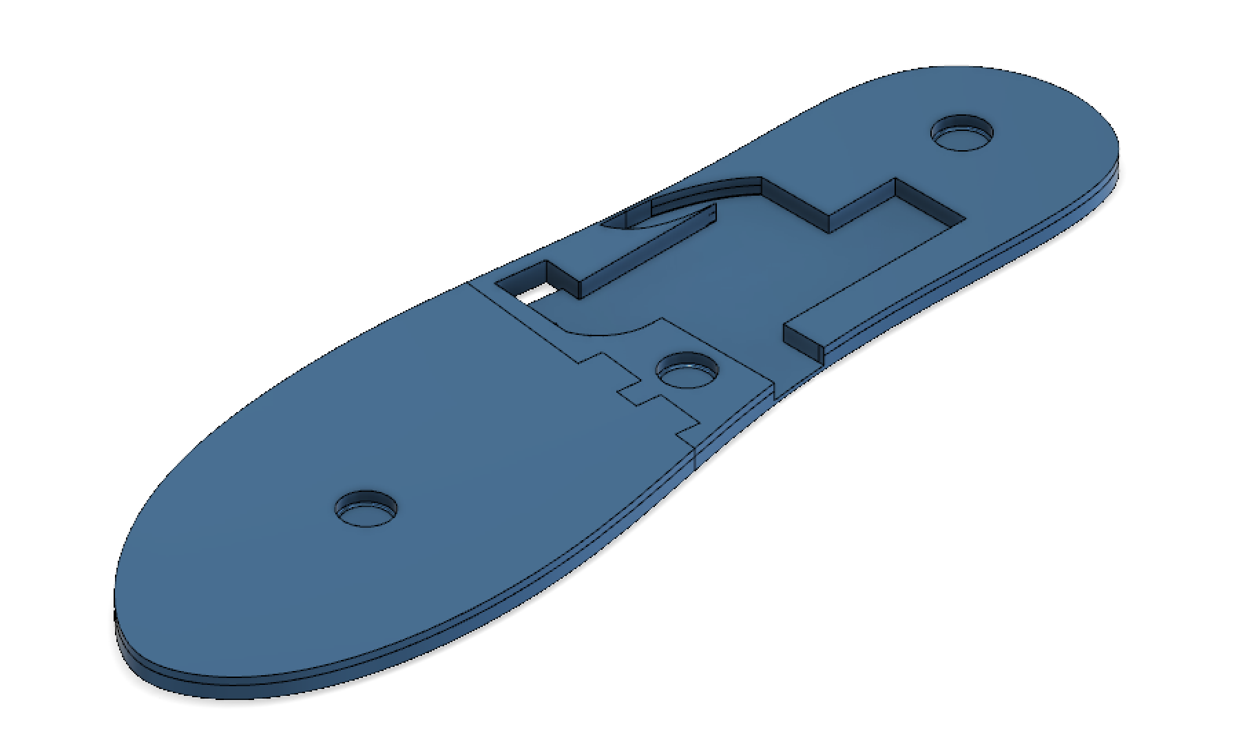
The middle layer of this design is for the motherboard. Since the motherboard was a single-layer board, it needed a total surface footprint of 2.00" by 1.50" plus additional room for connectors hanging off the board. As a result, it needed to be on its own layer or it would have interfered with the pressure sensors. The motherboard is placed in a recess with a depth of 0.0825" just ahead of the heel pressure sensor. Since the PCB width is 0.063" and the tallest components in the final assembly measure 0.1" above the top of the board, the total height of this recess is 0.173" to accommodate with 0.01" of additional headroom.

The top layer is purely structural and exists for provide a relatively comfortable surface for the user to walk on while hiding away the rest of the electronics. It has a total z-height of just 0.11" and includes small 0.01" bumps where the four pressure sensors are housed. The rendering is also black for the top layer since it will be produced from the Flexible V2 resin.

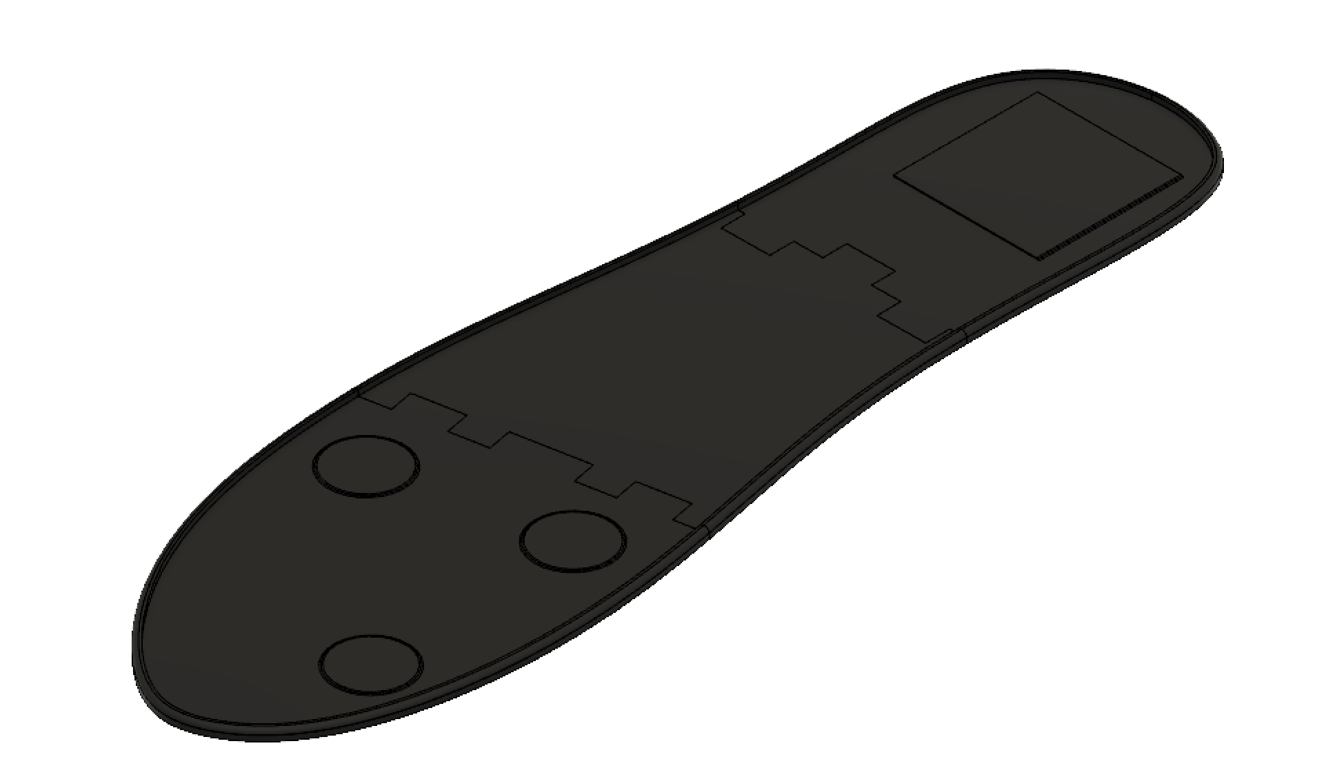
The total stackup height of the three layers was 0.43" which is thicker than the target 0.40", but still within the design specifications.

Signal Processing

For early graphs, the Arduino IDE built-in Serial Plotter was sufficient to receive incoming step data and generate a graph in real time. The persistence of "memory" in this graph was limited to approximately the previous 5 seconds that were visible on the graph at any given time. The Arduino plotter also did not present any way to change the default color set, line width, or other properties related to the graph displayed.

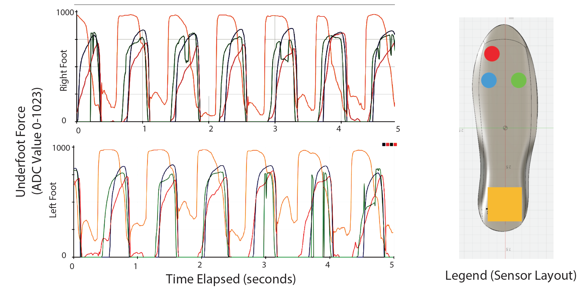
This graph shows the relative underfoot pressures measured by the force sensitive resistors during a regular walking pattern. This data clearly shows the distinction between ``step" moments where the pressure is high and non-step moments where the pressure is low.

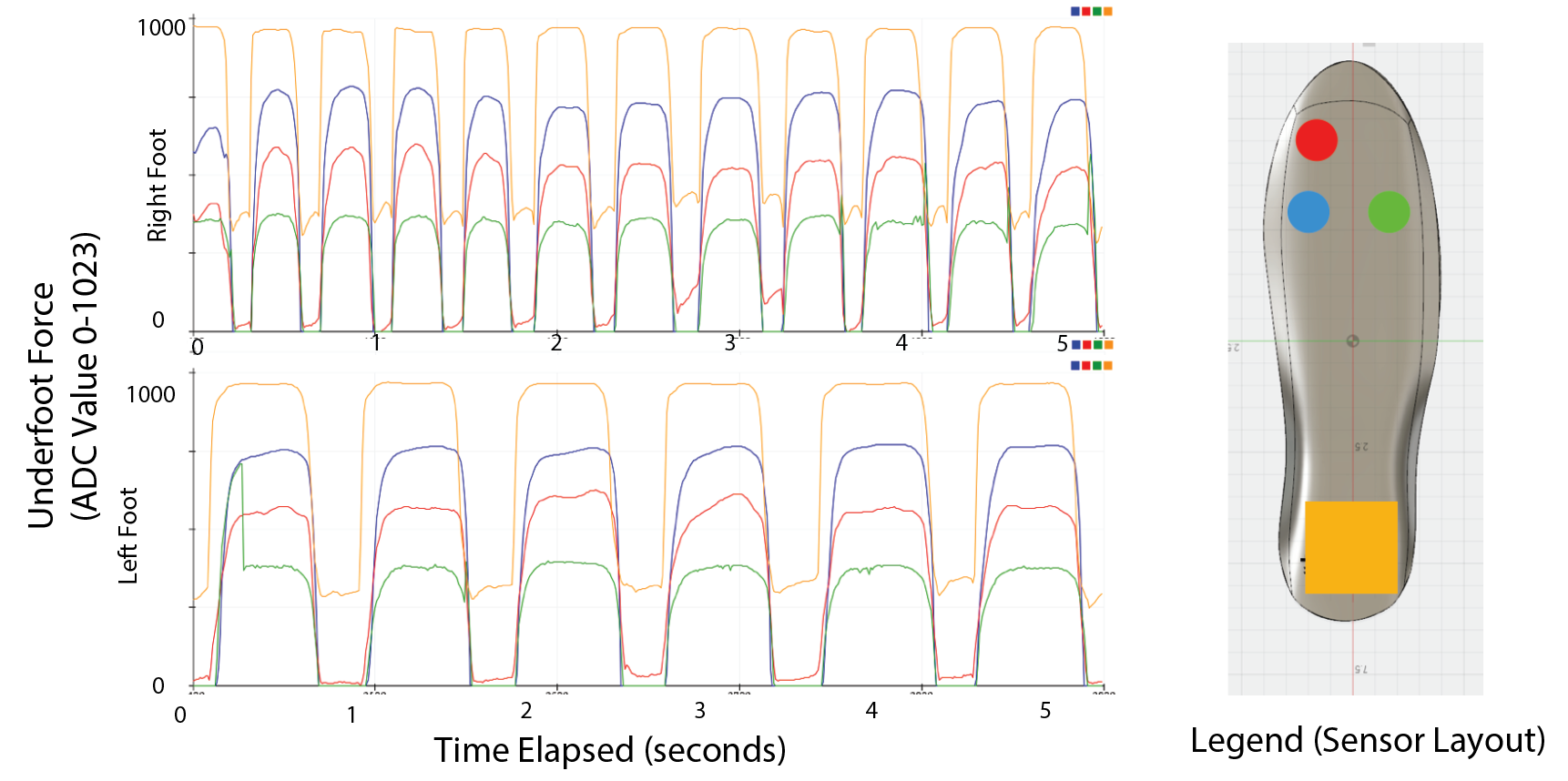
A similar distinction can be seen in graphs where the user is simply rocking back and forth without taking unique steps. The key distinction here is that the heel pressure (yellow line) does not lead the three measurements taken from the front of the foot, but rather is entirely within phase. This data is meaningful for later informing the step-counting algorithm.

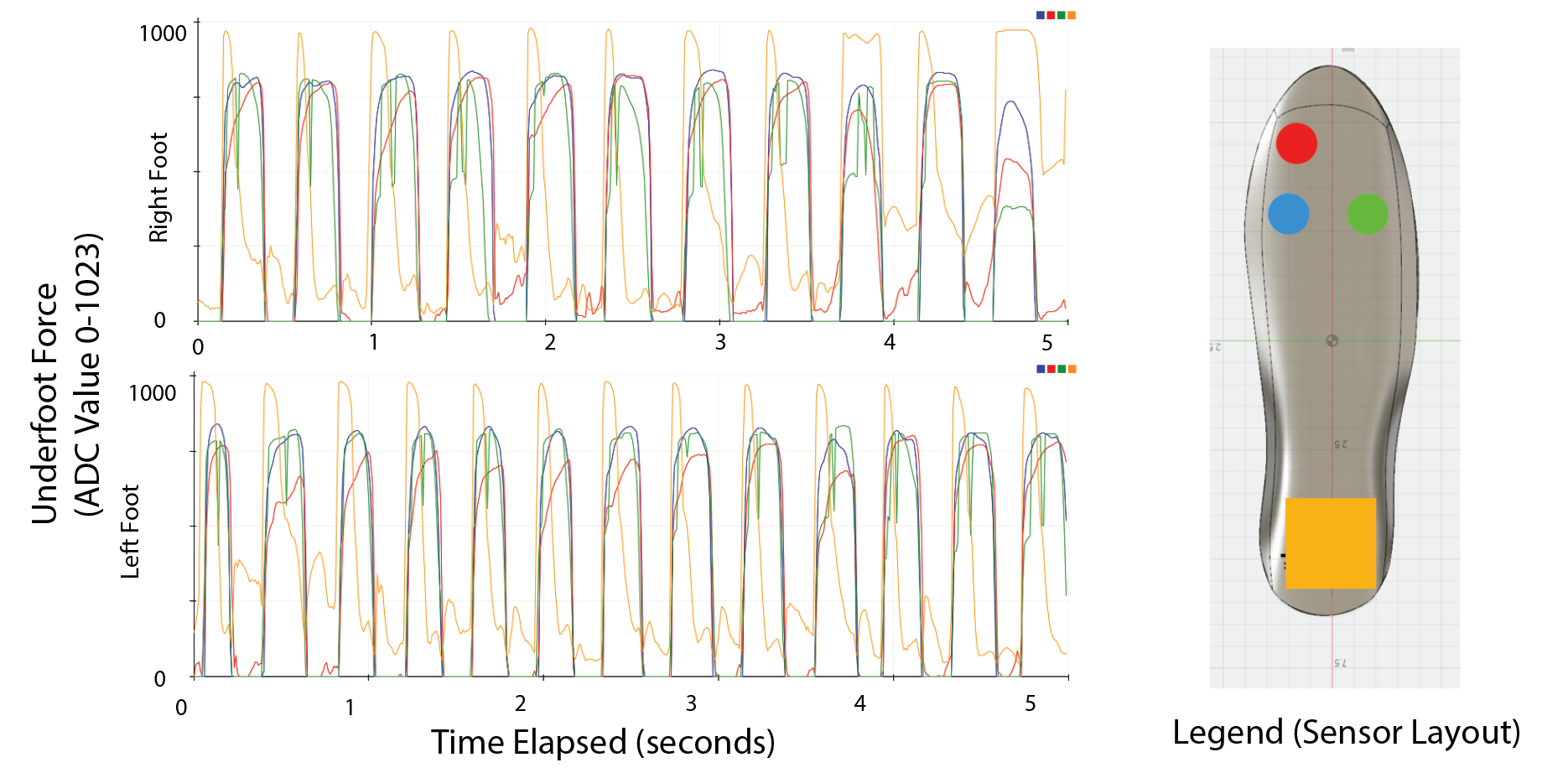
Similarly, running data was collected which can be thought of as higher frequency walking data. The running data helps define a minimum data sampling rate to ensure no steps are lost. In this case, a data frequency of 50 Hz was sufficient to capture the fasts steps resulting from running, which could be upwards of 8 steps in one second at higher speeds.

The Arduino IDE build-in serial plotter does not allow for data to be written to a file. Another serial monitor program called CoolTerm allows for output to be captured to a text file, so it was used to collect longer time-horizon data. CoolTerm also allowed for time-stamping of the data which, despite a timestamp resolution too low to capture times lower than on the order of seconds, was helpful in tracking the overall data-rate and sample time durations.

Data Filtering and Processing

The raw data collected from a wearer's step profile contained a high degree of noise due to the relatively high sampling rate of 50 Hz. The sample below shows a large amount of noise across 10 steps. It should be noted that, as in the previous sample of waling data, it is clear that the heel leads the sensors at the front of the foot.

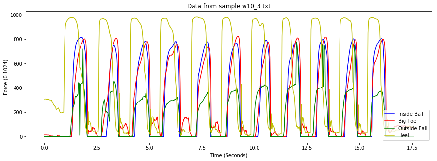
The raw 50 Hz data plotted here shows several examples of high frequency noise. The outside ball sensor (green) in particular shows large spikes in the first step of the sample data. In order to apply some sort of thresholding calculation to convert the raw step data into a binary format, high frequency noise like this must first be eliminated.

A low-pass filter in the form of a simple moving average was applied to the data to smooth out high frequency noise. In this implementation, the pressure value at a given time is the average of the pressure reading taken at that time averaged with some number n of values before that time. A good value of n is one that allows the maximum and minimum steady-state values of the data to remain unaffected while smoothing out higher frequencies in the transitions between.

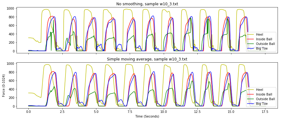
The figures below show examples of the processed data after smoothing with values n = 0, 5, 10, 20. For simplicity, only one of the four FSR measurements is shown to better demonstrate the effects of the simple moving average smoothing. As the n used for smoothing gets higher, the peaks in the data become more and more triangular.

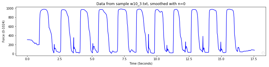
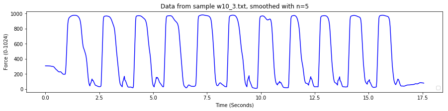
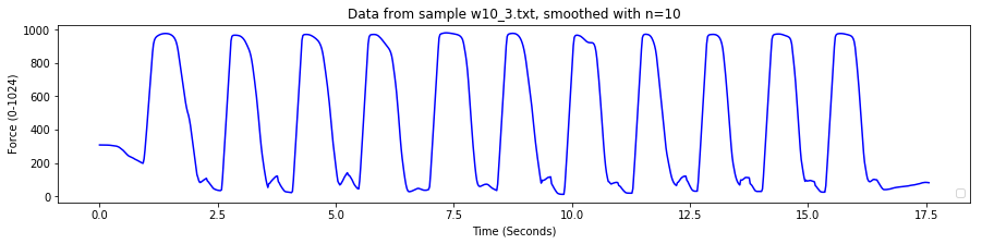
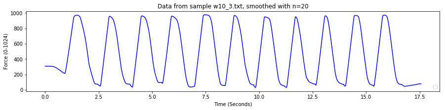
A smoothing value of n = 10 was chosen in order to strike a balance between filtering out as much noise as possible while still maintaining the peaks and valleys of faster movement patterns like running. This low-pass filter was applied to all four channels of data in order to eliminate the high frequency noise, as seen below.

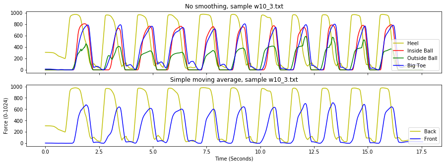
One trend across all samples of step data was that the three sensors at the front of the foot (inside ball, outside ball, and toe) were nearly always in phase while the heel was in a leading position. Furthermore, different terrain and environmental conditions could shift the relative distributions of weight in the front-of-foot sensors, but they would usually average out to the same value. In order to simplify the binary classification of the data, the three sensors at the front of the foot were averaged together after filtering. Instead of four pressure values, only two pressure values representing the front and back of the foot were considered.

The final step in processing the data was to convert the data into a set of binary values over time that could be fed into the step-counting algorithm. An asymmetric threshold system with hysteresis was set up to determine when to switch between the "stepped" and "in-the-air" states. This thresholding was applied to the "front" and "back" step data separately.

The algorithm worked by starting at the beginning of the data and stepping through forward in time. The "in-the-air" state was represented by a 0 and was where the system began. Successive values were checked against a threshold and, when a value exceeded 80% of the maximum value (determined on a separate pass through the data) the state of the system changed from "in the air" to "stepped".

Once in the "stepped" state, the threshold to change back to the "in-the-air" state required the pressure value to drop below 20% of the maximum value. This asymmetric thresholding ensured that steady-state values between 20% and 80% of the maximum value were not errantly counted as steps. This asymmetric thresholding allowed for rejection of standing and sitting steady-forces on the pressure sensors

Once this algorithm was run on the data set, the analog pressure values over time were converted to a set of digital pressure values over time that are visible in the figure below.

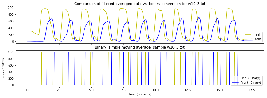
The resulting data had enough information for processing by a step-counting algorithm to output the health statistics specified in the project's sensor specification.

Step-counting Algorithm

The state of the pressure sensors in a shoe at any given time can be defined by the front sensors reading a 0 or 1 as well as the back sensor reading a 0 or 1. This gives four possible states of the system as shown below.

A finite state machine can be set up characterizing the flow of the system between states to determine when steps are counted. The finite state machine has four possible states at time n and the same four possible states at time n-1 meaning there are sixteen "transitions". Four of these are represent a transition from a state to itself - these are omitted. The other twelve transitions cover unique transitions between system states.

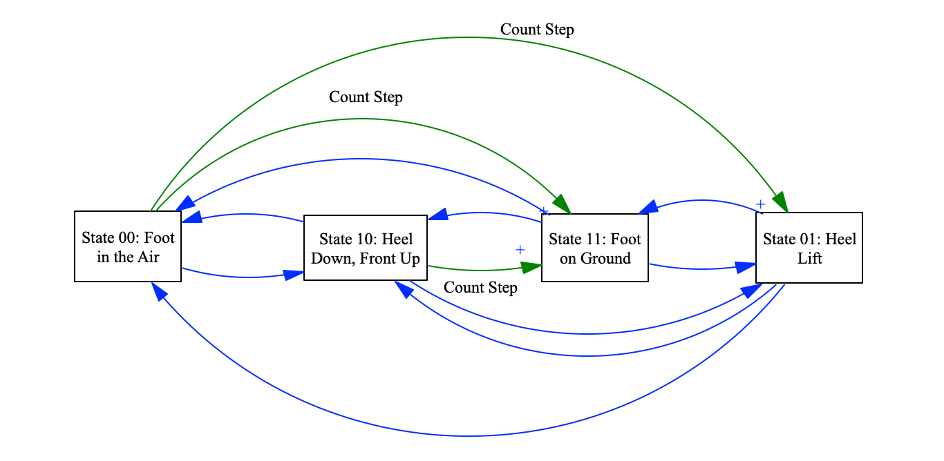
All twelve possible transitions are shown in the finite state diagram above with the states and the transitions documented. Three states shown in green are identified as the transitions on which a "step" should be counted and added to the total. A better representation of the physical meaning of each of the FSM transitions is shown below.

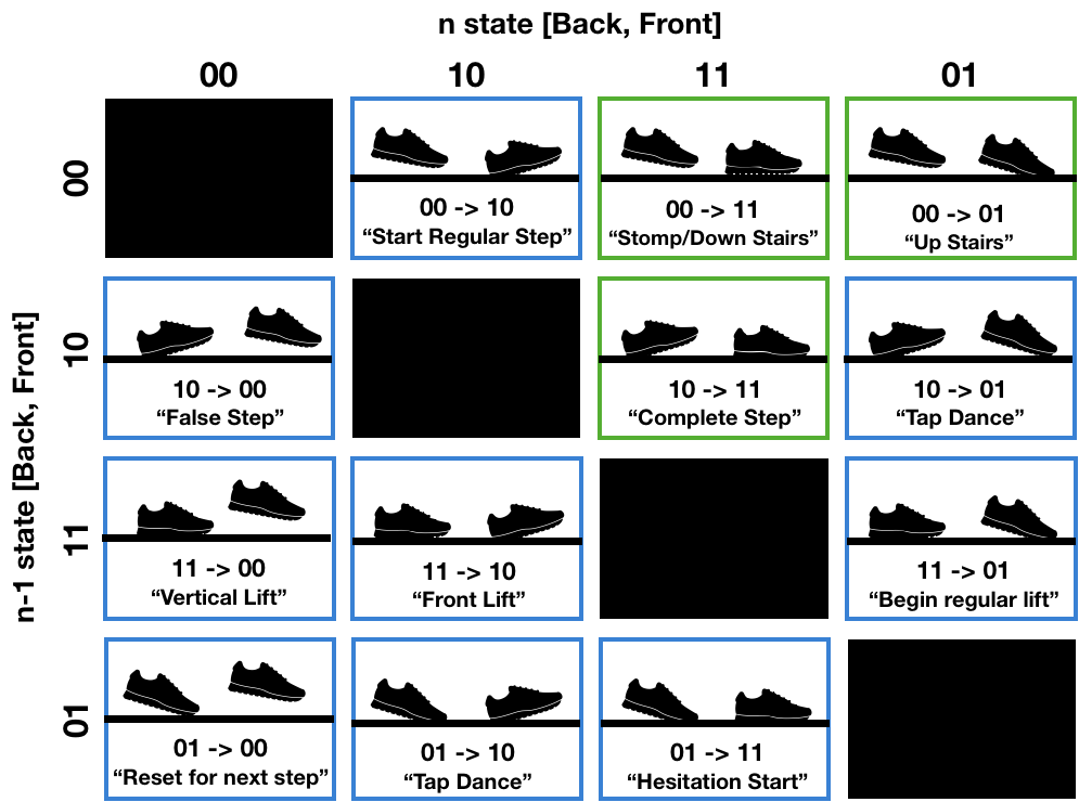
This FSM algorithm was tested against 20 samples of data from standard walking. The algorithm was very effective, successfully classifying 202 out of the 203 steps taken across all samples for a 99.51% success rate.

This page only captures a sampling of the work completed as part of this senior thesis project. The full thesis is available upon request or available to be checked out from the Harvard University Library System.